Understanding AI Fabric Architecture
An AI training fabric is the network that moves AllReduce traffic between thousands of GPUs. It looks like a spine-leaf CLOS at first glance — and structurally it is — but the way the components are wired, the bandwidth per host, and the operational rules underneath are different from any data-center fabric you've designed before. This page is the conceptual map of one.
At a glance
The rest of this page is a guided tour of that diagram. Skim the image first; the prose then walks each piece.
1. The components — a guided tour
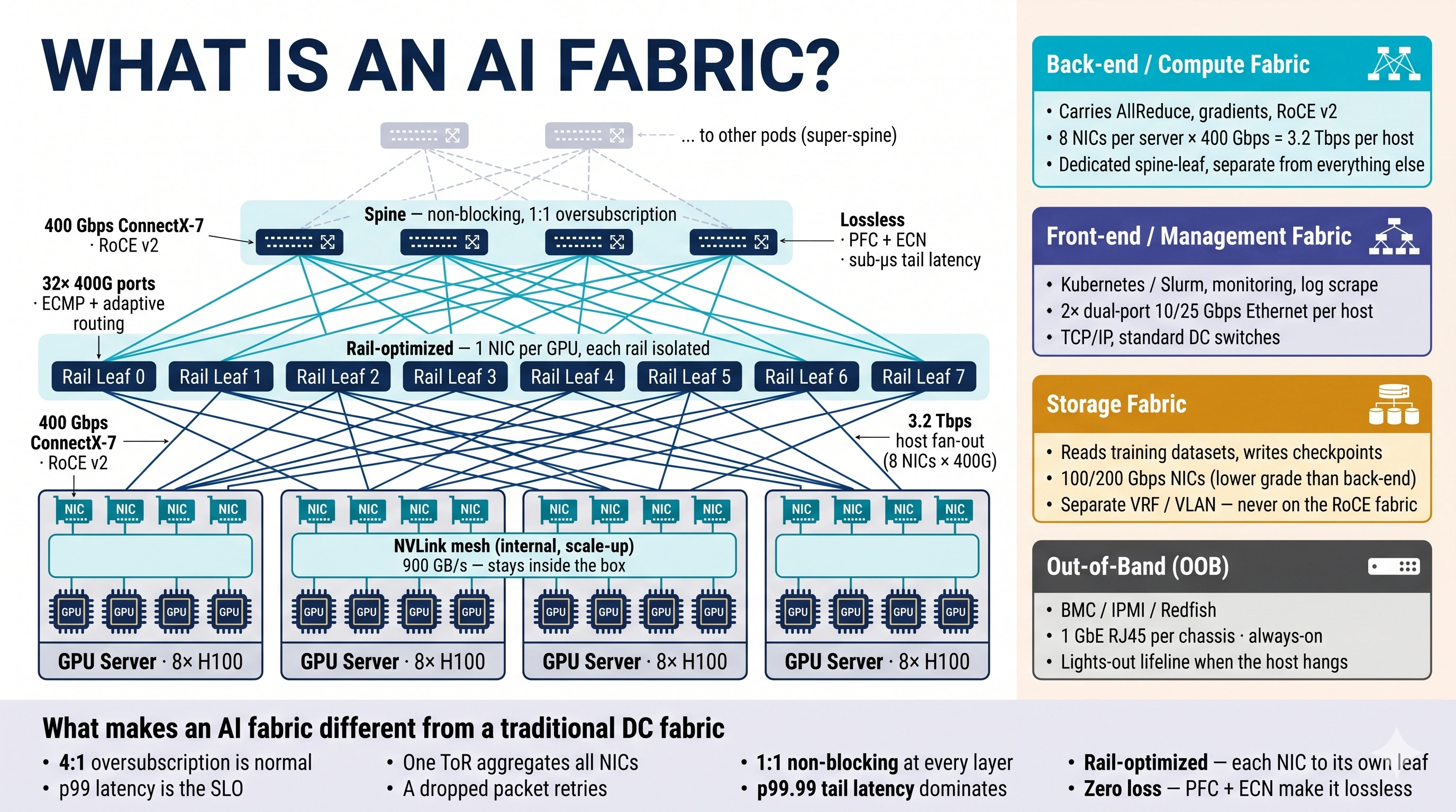
Read the diagram bottom to top.
GPU servers (bottom row). Each box is a single AI training host — typically 8 H100 GPUs on an HGX baseboard, plus 8 ConnectX-7 NICs, one NIC per GPU. Inside the chassis, the 8 GPUs talk to each other over an NVLink mesh at 900 GB/s through 4 NVSwitch chips. That traffic stays inside the box; it never reaches the fabric you're about to design.
Rail leaves (middle row). The structural break from a traditional DC. Instead of one ToR aggregating all 8 NICs on a server, each NIC lands on its own dedicated leaf — a "rail leaf." NIC 0 from every server connects to Rail Leaf 0; NIC 1 from every server connects to Rail Leaf 1; and so on. 8 NICs per server = 8 separate rail fabrics, each operationally independent. Same-index GPUs across the cluster are exactly one hop apart by design.
Spine (top row). Above the rail leaves, a non-blocking Clos. Every rail leaf connects to every spine, 1:1 oversubscription end-to-end — no bottlenecks anywhere on the back-end path. For pods larger than ~1K GPUs, a super-spine tier stitches multiple pods together.
The whole stack has one job: move AllReduce traffic between same-index GPUs with sub-microsecond tail latency and zero packet loss.
2. The four fabrics in one cluster
The diagram's right column makes this explicit: one AI training cluster has four physically separate networks, not one. They share the same datacenter floor but never share switches.
| Fabric | Carries | Speed | Switches |
|---|---|---|---|
| Back-end / Compute (cyan) | AllReduce, gradients · RoCE v2 · the path this whole curriculum is about | 400 Gbps per NIC · 3.2 Tbps host fan-out | Dedicated spine-leaf, rail-optimized |
| Front-end / Management (indigo) | Kubernetes/Slurm, monitoring scrape, log shipping · TCP/IP | 10–25 Gbps, 2× dual-port per host | Standard DC switches |
| Storage (amber) | Dataset reads, checkpoint writes | 100/200 Gbps | Separate VRF / VLAN — never on the RoCE fabric |
| Out-of-Band (OOB) (grey) | BMC, IPMI, Redfish · lights-out management | 1 GbE always-on | Separate small management switches |
The rule: back-end and front-end never share a switch. The reason is microseconds — a storage burst or a monitoring scrape mixed onto the RoCE fabric eats headroom the AllReduce was counting on, and tail latency blows up. Vendors enforce this with separate ToRs.
3. What makes it different from a traditional DC fabric
The bottom band of the diagram is the executive summary. Same CLOS shape, four rules flipped:
- 4:1 oversubscription is normal in the DC you know. 1:1 non-blocking at every layer is the AI fabric rule.
- p99 latency is the DC SLO. p99.99 tail latency is what dominates an AI fabric — one slow link stalls thousands of GPUs.
- One ToR aggregates all server NICs in a traditional design. Rail-optimized spreads each NIC to its own leaf.
- A dropped packet retries on a TCP fabric. Zero loss is mandatory on an AI fabric — RDMA has no graceful retransmit.
The five-page rest of this chapter unpacks why each rule flipped and how you build for it.
4. The same view, interactive
If you want to flip between "traditional DC" and "AI fabric" rule-by-rule, the embedded component below does exactly that — same CLOS shape, four rules animated.
A traditional DC fabric and an AI fabric look identical from across the room — spine-leaf, BGP underlay, ECMP. Up close, four design rules flip. Each animation below shows one of them.
What stays the same, what changes
| Element | Traditional DC | AI Fabric |
|---|---|---|
| Topology | Spine-leaf CLOS | Spine-leaf CLOS ✓ same shape |
| Underlay | eBGP | eBGP ✓ same |
| Routing | ECMP (5-tuple hash) | ECMP ✓ same — but the failure modes change |
| Oversubscription | 4:1 typical | 1:1 non-blocking |
| NICs per server | 1–2 bonded | 8 — one per GPU rail |
| Traffic shape | Many short flows, statistically independent | Few huge elephant flows, synchronized |
| Tolerance for loss | TCP recovers | RDMA NACK = idle GPUs |
1. Oversubscription
Traditional DC fabrics oversubscribe — a 32-port leaf has only 8 spine uplinks (4:1), because most servers are mostly idle. AI workloads are the opposite: every NIC pushes line-rate, simultaneously. That's why AI fabrics buy enough spine ports for 1:1 — and the spend is justified because tail latency = idle GPUs = wasted money.
2. Rail-optimized topology
A traditional server has one or two NICs, both on the same ToR. An AI server has 8 NICs, each going to its own dedicated leaf — one per GPU. Each "rail" is an independent fabric end to end. A link failure on rail 4 only impacts GPU 4; the other 7 GPUs keep training. That's the blast-radius story.
3. Hash polarization
ECMP hashes the 5-tuple to spread flows evenly. With diverse traffic (web, API, DB), the law of large numbers makes this work great. With synchronized AllReduce — every GPU sending identically shaped flows at the same instant — many flows hash to the same path. One spine link saturates while three sit idle. This is the failure mode that destroys training throughput.
4. ECMP and link failures
When a spine link goes down, ECMP rehashes the affected flows onto the survivors. This is fine for TCP — the kernel retransmits. For RDMA RC, in-flight packets on the now-dead path arrive out of order on a surviving path; the receiver's RNIC sees a PSN gap and sends a NACK. The sender retransmits the whole window. Multiply by every flow on the dead link and you get a short NACK storm.
What hyperscalers do about it: rail isolation limits blast radius; adaptive routing and packet spraying (BlueField, Spectrum-X, Tomahawk-5) sidestep hash polarization; faster link-down detection (sub-millisecond LFI / BFD) and pre-computed FRR paths shrink the NACK window. Net result: a single spine link failure becomes a brief dip, not an outage.
The deeper details — pod sizing, super-spine, oversub math, mitigations for hash polarization — live in the three pages after this one.
5. Where this chapter goes
The image and this page are the conceptual map. The remaining pages each take one piece of it deep:
- Design Options — the four design patterns (ROD, RUD, Scheduled, Multi-Planar) and how to pick.
- Rail-Optimized Design — deep dive on the default pattern. Pod sizing, blast radius, NCCL ring isolation.
- Cluster Sizing & Cabling — reference designs at 256 → 100K GPUs, switch radix, optics, day-1 install reality.
The next chapter — 04. Load Balancing in AI Fabrics — is the dedicated deep-dive on how the back-end fabric actually moves bytes once this design is in place. ECMP, hash polarization, DLB, GLB, TELB, and a live simulator.
💡 What you should remember
| 🏗️ | An AI fabric IS spine-leaf CLOS | The topology shape is familiar. Leaves, spines, super-spines, eBGP underlay — all there. |
| 🛤️ | Rail-optimized is the structural break | Each GPU's NIC lands on its own dedicated leaf. 8 NICs per host = 8 separate rail fabrics. |
| 🧵 | Four fabrics, one cluster | Back-end (RoCE) · Front-end (mgmt) · Storage · OOB. Never share switches. |
| 🚦 | Back-end carries AllReduce; nothing else | 3.2 Tbps host fan-out, 1:1 non-blocking, lossless. The other three fabrics exist so the back-end stays clean. |
| ⏱️ | p99.99 tail latency is the only latency | One slow link stalls thousands of GPUs. Design for the worst link, not the average. |
Next: Design Options → — the four fabric design patterns and how to pick between them. The catalog before the deep dives.